5  Wealth indexes

This section documents the process of reconstructing and analyzing wealth indexes for a forthcoming study focusing on rural populations in Madagascar. Wealth indexes, particularly the wealth index factor scores, are critical for assessing household living standards and analyzing inequalities.

The wealth index, provided in DHS, is constructed using principal components analysis on household characteristics such as asset ownership, housing materials, and access to water and sanitation facilities. We want a centile classification specific to rural households.

5.1 Verification that rural wealth centiles can be derived from existing DHS data

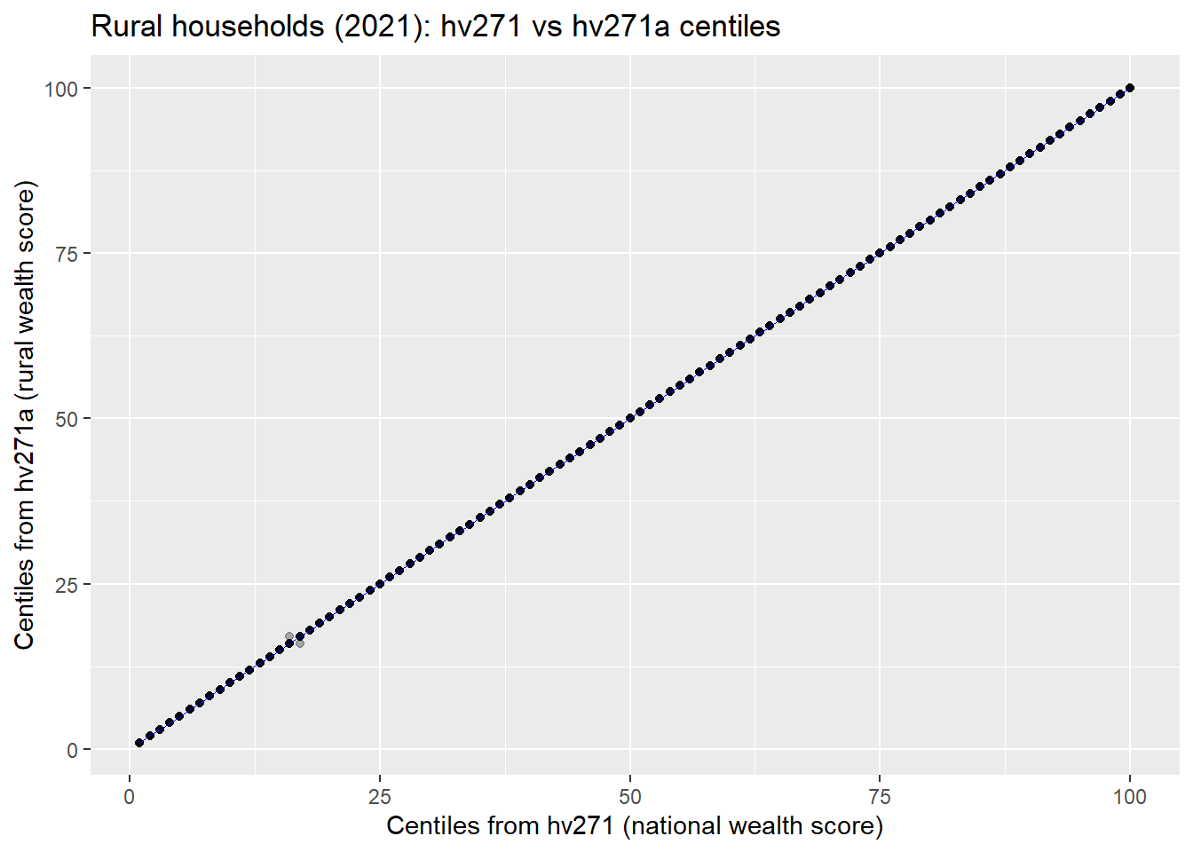
We first check whether the centile classification of households is consistent between the national wealth score (hv271) and the rural-specific wealth score (hv271a). The comparison is done for rural households in the 2021 DHS. Both indices are transformed into centiles, and we examine their agreement through simple proportions, correlation, and a scatterplot.

library(tidyverse)
library(haven)
library(survey)

hh21 <- read_dta("data/raw/dhs/DHS_2021/MDHR81DT/MDHR81FL.DTA")

# Rural only
hh21_rur <- hh21 %>%
  filter(hv025 == 2) %>%
  transmute(
    hv001, hv002, hv005,
    c_hv271  = ntile(hv271,  100),
    c_hv271a = ntile(hv271a, 100)
  )

# Centile agreement
mean(hh21_rur$c_hv271 == hh21_rur$c_hv271a, na.rm = TRUE)

[1] 0.9998698

cor.test(hh21_rur$c_hv271, hh21_rur$c_hv271a,
         method = "spearman", use = "complete.obs")

    Spearman's rank correlation rho

data:  hh21_rur$c_hv271 and hh21_rur$c_hv271a
S = 47437, p-value < 2.2e-16
alternative hypothesis: true rho is not equal to 0
sample estimates:
      rho 
0.9999999 

#  Scatterplot with both axes
ggplot(hh21_rur, aes(x = c_hv271, y = c_hv271a)) +
  geom_point(alpha = 0.3) +
  geom_smooth(method = "lm", se = FALSE, linewidth = 0.3, color = "blue") +
  labs(
    title = "Rural households (2021): hv271 vs hv271a centiles",
    x = "Centiles from hv271 (national wealth score)",
    y = "Centiles from hv271a (rural wealth score)"
  )

The results show near-perfect agreement between the two indices, confirming that the national wealth index can be used directly to reconstruct rural centiles, without loss of consistency. This greatly simplifies the treatment of earlier surveys (MIS 2011, 2013, 2016), where domain-specific wealth scores are not provided.

5.2 Construction of rural wealth centiles across DHS surveys

For comparability over time, we rely directly on the DHS wealth score (hv271) available in each household dataset. In the 1997 DHS, the wealth index is stored separately and must be merged by household identifier. For subsequent surveys (2008–2021), it is included directly in the household file.

We then define a single function that filters rural households and computes both unweighted centiles (using ntile()) and weighted centiles that respect the DHS survey design. Weighted centiles are calculated with the survey package using the household sampling weights (hv005). To avoid problems with ties in the weighted quantile thresholds, we add an infinitesimal offset to ensure strictly increasing cut-points.

# In 1997, the wealth indexes are stored in a separate file
wi97 <- read_dta("data/raw/dhs/DHS_1997/MDWI31DT/MDWI31FL.DTA") %>%
  select(whhid, hv271 = wlthindf) %>%
  mutate(whhid = str_trim(whhid, side = "left"))
hh97 <- read_dta("data/raw/dhs/DHS_1997/MDHR31DT/MDHR31FL.DTA") %>%
  select(hv001, hv002, hv005, hv025) %>%
  mutate(whhid = paste0(hv001, 
                        str_pad(as.character(hv002), width = 2, side = "left", 
                                pad = " ")))%>%
  inner_join(wi97, by = "whhid")
# Load the others
hh08 <- read_dta("data/raw/dhs/DHS_2008/MDHR51DT/MDHR51FL.DTA") %>%
  select(hv001, hv002, hv005, hv025, hv271)
hh11 <- read_dta("data/raw/dhs/DHS_2011/MDHR61DT/MDHR61FL.DTA") %>%
  select(hv001, hv002, hv005, hv025, hv271)
hh13 <- read_dta("data/raw/dhs/DHS_2013/MDHR6ADT/MDHR6AFL.DTA") %>%
  select(hv001, hv002, hv005, hv025, hv271)
hh16 <- read_dta("data/raw/dhs/DHS_2016/MDHR71DT/MDHR71FL.DTA") %>%
  select(hv001, hv002, hv005, hv025, hv271)
hh21 <- read_dta("data/raw/dhs/DHS_2021/MDHR81DT/MDHR81FL.DTA") %>%
  select(hv001, hv002, hv005, hv025, hv271)


rural_centiles <- function(df) {
  # filter rural only
  df_rur <- df %>% filter(hv025 == 2)

  # weighted centiles
  df_rur <- df_rur %>% mutate(.w = hv005 / 1e6)
  des <- svydesign(ids = ~hv001, weights = ~.w, data = df_rur)

  qs <- svyquantile(~hv271, des,
                    quantiles = seq(0.01, 1, 0.01),
                    ci = FALSE, na.rm = TRUE)
  # Avoid ties for weighted centiles
  thr <- as.numeric(qs[[1]]) + seq_along(qs[[1]]) * 1e-10

  df_rur %>%
    mutate(
      wealth_centile_rural_weighted = 
        cut(hv271, breaks = c(-Inf, thr),
            labels = 1:100, include.lowest = TRUE, right = TRUE) %>% 
        as.integer(),
      wealth_centile_rural_simple = ntile(hv271, 100)
    ) %>%
    select(-.w)
}


add_zscore_from_centile <- function(df, centile_col, cluster_col, zscore_col = "zscore_wealth") {
  stats <- df %>%
    group_by(.data[[cluster_col]]) %>%
    summarise(m = mean(.data[[centile_col]], na.rm = TRUE),
              s = sd(.data[[centile_col]],   na.rm = TRUE),
              .groups = "drop")
  df %>%
    left_join(stats, by = cluster_col) %>%
    mutate(!!zscore_col := ifelse(!is.na(s) & s > 0,
                                  abs(.data[[centile_col]] - m) / s, NA_real_)) %>%
    select(-m, -s)
}

# Apply
hh97_rur <- rural_centiles(hh97) %>%
  add_zscore_from_centile("wealth_centile_rural_weighted", "hv001")
hh08_rur <- rural_centiles(hh08) %>%
  add_zscore_from_centile("wealth_centile_rural_weighted", "hv001")
hh11_rur <- rural_centiles(hh11) %>%
  add_zscore_from_centile("wealth_centile_rural_weighted", "hv001")
hh13_rur <- rural_centiles(hh13) %>%
  add_zscore_from_centile("wealth_centile_rural_weighted", "hv001")
hh16_rur <- rural_centiles(hh16) %>%
  add_zscore_from_centile("wealth_centile_rural_weighted", "hv001")
hh21_rur <- rural_centiles(hh21) %>%
  add_zscore_from_centile("wealth_centile_rural_weighted", "hv001")

# Write
write_rds(hh97_rur, "data/derived/hh_1997_rural_simpler.rds")
write_rds(hh08_rur, "data/derived/hh_2008_rural_simpler.rds")
write_rds(hh21_rur, "data/derived/hh_2021_rural_simpler.rds")
write_rds(hh16_rur, "data/derived/hh_2016_rural_simpler.rds")
write_rds(hh13_rur, "data/derived/hh_2013_rural_simpler.rds")
write_rds(hh11_rur, "data/derived/hh_2011_rural_simpler.rds")

The rural wealth centiles are now computed consistently across survey types and years, using the national wealth index as a starting point, with (wealth_centile_rural_weighted) and without (wealth_centile_rural_simple) survey wheighing.